All I Overfitting for Overfitting is Overfitting
A couple of weeks ago I used Forecast Forge to build a forecast for the number of pageviews of the “All I Want for Christmas is You” wikipedia page in the run-up to Christmas.
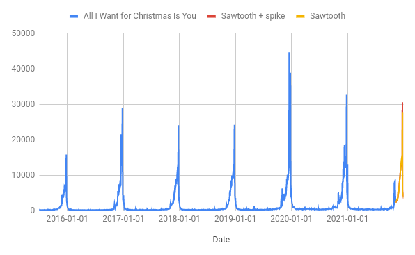
pageviews for the “All I Want For Christmas is You” wikipedia page will peak on 24th December close to 30k
This forecast “looks” good - it has the peak roughly when we’d expect it and the magnitude is comparable with previous years. It passes the smell test, but I am still concerned about whether it predicts the size of the peak correctly. As you can see from the chart, the peak in 2019 was way higher than any of the preceeding years and getting this right is the most important part of my prediction. How can we tell in advance what kind of peak there is going to be?
My hypothesis is that the peak in 2019 was driven by the re-release of the Merry Christmas album; something that would have been known about on the 8th November 2019 when the corresponding 2019 forecast would have been made. If I was a Mariah Carey expert I would be able to include broader information like this in a regression column; probably by giving each December a mark out of 10 for how much Mariahhad going on that year.
But I am not a Mariah Carey expert so I don’t trust my intuition on this; I need some hard data to work with here that might give me an inkling of whether or not she is having a big year.
The first idea that sprang to mind was that it might be possible to use traffic data from other wikipedia pages for this. The challenge is then to find which pages are a leading indicator of Christmas traffic for “All I Want for Christmas is You”.
Doing this analysis for all pages on Wikipedia would make the challenge more about dealing with big data so instead I first need to select a subset of pages for first analysis. All the pages that link to “All I Want for Christmas is You” seems like a good starting point. You can see a list of these using the linksto: operator and download the pageview data from the Massviews tool.
The rest of this post will be me analysing this data and trying (failing!) to use it to make a better forecast.
You can download the Jupyter Notebook from here. All the code an explanations are also included below.
First let’s load the data into python
import pandas as pd

inlinks = pd.read_csv("https://www.forecastforge.com/files/massviews-20150701-20211116.csv",
                      # Need to set this otherwise cloudflare (I think?) 403's the pandas request
                      storage_options = {'User-Agent': 'Pandas!'})
inlinks| Title | 2015-07-01 | 2015-07-02 | 2015-07-03 | 2015-07-04 | 2015-07-05 | 2015-07-06 | 2015-07-07 | 2015-07-08 | 2015-07-09 | … | 2021-11-07 | 2021-11-08 | 2021-11-09 | 2021-11-10 | 2021-11-11 | 2021-11-12 | 2021-11-13 | 2021-11-14 | 2021-11-15 | 2021-11-16 | |
|---|---|---|---|---|---|---|---|---|---|---|---|---|---|---|---|---|---|---|---|---|---|
| 0 | Justin Bieber | 11212 | 11419 | 10973 | 10816 | 10737 | 11675 | 14246 | 13780 | 12273 | … | 13804 | 13002 | 12540 | 13343 | 14681 | 13842 | 12980 | 13267 | 14624.0 | 14028.0 |
| 1 | Millie Bobby Brown | 0 | 0 | 0 | 0 | 0 | 0 | 0 | 0 | 0 | … | 14229 | 11248 | 9497 | 8314 | 8197 | 8453 | 12435 | 11840 | 9445.0 | 9979.0 |
| 2 | Mariah Carey | 9832 | 14382 | 10988 | 9595 | 9428 | 9329 | 8735 | 13985 | 10900 | … | 16638 | 14650 | 13315 | 13851 | 15706 | 14629 | 12662 | 13895 | 13326.0 | 10419.0 |
| 3 | Fifth Harmony | 11649 | 11674 | 10864 | 10733 | 11292 | 12147 | 12247 | 12316 | 11701 | … | 2385 | 2071 | 2169 | 2334 | 2098 | 2151 | 2244 | 2091 | 2104.0 | 1918.0 |
| 4 | Jenna Dewan | 13182 | 26490 | 21592 | 16881 | 14074 | 16984 | 12811 | 11701 | 10932 | … | 3598 | 4857 | 3929 | 3307 | 2906 | 2582 | 2590 | 3292 | 5002.0 | 4402.0 |
| … | … | … | … | … | … | … | … | … | … | … | … | … | … | … | … | … | … | … | … | … | … |
| 628 | Ngayong Pasko | 0 | 0 | 0 | 0 | 0 | 0 | 0 | 0 | 0 | … | 1 | 4 | 1 | 0 | 4 | 2 | 0 | 2 | 1.0 | 1.0 |
| 629 | Česko Slovenská SuperStar (season 4) | 0 | 0 | 0 | 0 | 0 | 0 | 0 | 0 | 0 | … | 4 | 8 | 3 | 4 | 2 | 2 | 0 | 2 | 1.0 | 7.0 |
| 630 | Mr. Vocalist X’Mas | 0 | 0 | 0 | 0 | 0 | 0 | 0 | 0 | 0 | … | 3 | 2 | 2 | 0 | 0 | 1 | 3 | 0 | 3.0 | 1.0 |
| 631 | 24 Hours (Agnes song) | 0 | 0 | 0 | 0 | 0 | 0 | 0 | 0 | 0 | … | 19 | 14 | 15 | 10 | 9 | 9 | 8 | 6 | 14.0 | 4.0 |
| 632 | We Were Born for This | 0 | 0 | 0 | 0 | 0 | 0 | 0 | 0 | 0 | … | 3 | 1 | 4 | 4 | 3 | 4 | 6 | 1 | 3.0 | 12.0 |
633 rows × 2332 columns
This looks OK, but I would prefer it if each page was a separate column with a row for each day
inlinks = inlinks.transpose()
## Column names are in the first row
inlinks.columns = inlinks.iloc[0]
## Delete the first row
inlinks = inlinks.drop(["Title"])
inlinks| Title | Justin Bieber | Millie Bobby Brown | Mariah Carey | Fifth Harmony | Jenna Dewan | Love Actually | Michael Bublé | Despacito | Tori Kelly | Hallelujah (Leonard Cohen song) | … | Colleen Madden | List of Tawag ng Tanghalan finalists (season 3) | List of top 10 singles for 2018 in Australia | The Masked Singer (Bulgarian season 1) | List of Billboard Global 200 number ones of 2021 | Ngayong Pasko | Česko Slovenská SuperStar (season 4) | Mr. Vocalist X’Mas | 24 Hours (Agnes song) | We Were Born for This |
|---|---|---|---|---|---|---|---|---|---|---|---|---|---|---|---|---|---|---|---|---|---|
| 2015-07-01 | 11212 | 0 | 9832 | 11649 | 13182 | 2014 | 2129 | 0 | 12672 | 2091 | … | 0 | 0 | 0 | 0 | 0 | 0 | 0 | 0 | 0 | 0 |
| 2015-07-02 | 11419 | 0 | 14382 | 11674 | 26490 | 2409 | 2628 | 0 | 10764 | 2239 | … | 0 | 0 | 0 | 0 | 0 | 0 | 0 | 0 | 0 | 0 |
| 2015-07-03 | 10973 | 0 | 10988 | 10864 | 21592 | 2532 | 2350 | 0 | 8501 | 2290 | … | 0 | 0 | 0 | 0 | 0 | 0 | 0 | 0 | 0 | 0 |
| 2015-07-04 | 10816 | 0 | 9595 | 10733 | 16881 | 2514 | 2195 | 0 | 7252 | 2643 | … | 0 | 0 | 0 | 0 | 0 | 0 | 0 | 0 | 0 | 0 |
| 2015-07-05 | 10737 | 0 | 9428 | 11292 | 14074 | 2445 | 2344 | 0 | 6113 | 2675 | … | 0 | 0 | 0 | 0 | 0 | 0 | 0 | 0 | 0 | 0 |
| … | … | … | … | … | … | … | … | … | … | … | … | … | … | … | … | … | … | … | … | … | … |
| 2021-11-12 | 13842 | 8453 | 14629 | 2151 | 2582 | 4978 | 7419 | 1089 | 1088 | 1801 | … | 0 | 0 | 1 | 21 | 73 | 2 | 2 | 1 | 9 | 4 |
| 2021-11-13 | 12980 | 12435 | 12662 | 2244 | 2590 | 6175 | 4041 | 1181 | 1272 | 1947 | … | 1 | 1 | 1 | 27 | 74 | 0 | 0 | 3 | 8 | 6 |
| 2021-11-14 | 13267 | 11840 | 13895 | 2091 | 3292 | 7413 | 3608 | 971 | 2016 | 2002 | … | 0 | 3 | 4 | 15 | 61 | 2 | 2 | 0 | 6 | 1 |
| 2021-11-15 | 14624.0 | 9445.0 | 13326.0 | 2104.0 | 5002.0 | 6195.0 | 3051.0 | 1066.0 | 1057.0 | 1709.0 | … | 0.0 | 3.0 | 2.0 | 4.0 | 76.0 | 1.0 | 1.0 | 3.0 | 14.0 | 3.0 |
| 2021-11-16 | 14028.0 | 9979.0 | 10419.0 | 1918.0 | 4402.0 | 6276.0 | 3255.0 | 960.0 | 1225.0 | 1524.0 | … | 1.0 | NaN | 1.0 | 13.0 | 67.0 | 1.0 | 7.0 | 1.0 | 4.0 | 12.0 |
2331 rows × 633 columns
Much better!
Now load the “All I Want for Christmas is You” pageview data
alliwant = pd.read_csv("https://www.forecastforge.com/files/pageviews-20150701-20211108.csv",
                      storage_options = {'User-Agent': 'Pandas!'})
alliwant| Date | All I Want for Christmas Is You | |
|---|---|---|
| 0 | 2015-07-01 | 189 |
| 1 | 2015-07-02 | 248 |
| 2 | 2015-07-03 | 179 |
| 3 | 2015-07-04 | 208 |
| 4 | 2015-07-05 | 245 |
| … | … | … |
| 2318 | 2021-11-04 | 4103 |
| 2319 | 2021-11-05 | 3556 |
| 2320 | 2021-11-06 | 3192 |
| 2321 | 2021-11-07 | 3046 |
| 2322 | 2021-11-08 | 2760 |
2323 rows × 2 columns
Match the timeseries up by joining the dataframes together
## Default is inner join so rows match up
all_series = alliwant.join(inlinks, on="Date")
all_series = all_series.set_index("Date")
all_series| All I Want for Christmas Is You | Justin Bieber | Millie Bobby Brown | Mariah Carey | Fifth Harmony | Jenna Dewan | Love Actually | Michael Bublé | Despacito | Tori Kelly | … | Colleen Madden | List of Tawag ng Tanghalan finalists (season 3) | List of top 10 singles for 2018 in Australia | The Masked Singer (Bulgarian season 1) | List of Billboard Global 200 number ones of 2021 | Ngayong Pasko | Česko Slovenská SuperStar (season 4) | Mr. Vocalist X’Mas | 24 Hours (Agnes song) | We Were Born for This | |
|---|---|---|---|---|---|---|---|---|---|---|---|---|---|---|---|---|---|---|---|---|---|
| Date | |||||||||||||||||||||
| 2015-07-01 | 189 | 11212 | 0 | 9832 | 11649 | 13182 | 2014 | 2129 | 0 | 12672 | … | 0 | 0 | 0 | 0 | 0 | 0 | 0 | 0 | 0 | 0 |
| 2015-07-02 | 248 | 11419 | 0 | 14382 | 11674 | 26490 | 2409 | 2628 | 0 | 10764 | … | 0 | 0 | 0 | 0 | 0 | 0 | 0 | 0 | 0 | 0 |
| 2015-07-03 | 179 | 10973 | 0 | 10988 | 10864 | 21592 | 2532 | 2350 | 0 | 8501 | … | 0 | 0 | 0 | 0 | 0 | 0 | 0 | 0 | 0 | 0 |
| 2015-07-04 | 208 | 10816 | 0 | 9595 | 10733 | 16881 | 2514 | 2195 | 0 | 7252 | … | 0 | 0 | 0 | 0 | 0 | 0 | 0 | 0 | 0 | 0 |
| 2015-07-05 | 245 | 10737 | 0 | 9428 | 11292 | 14074 | 2445 | 2344 | 0 | 6113 | … | 0 | 0 | 0 | 0 | 0 | 0 | 0 | 0 | 0 | 0 |
| … | … | … | … | … | … | … | … | … | … | … | … | … | … | … | … | … | … | … | … | … | … |
| 2021-11-04 | 4103 | 12832 | 8495 | 18005 | 2393 | 3147 | 2783 | 2875 | 973 | 1525 | … | 0 | 1 | 1 | 5 | 0 | 0 | 2 | 1 | 6 | 4 |
| 2021-11-05 | 3556 | 12473 | 7724 | 18080 | 2206 | 2789 | 4056 | 2925 | 992 | 1341 | … | 3 | 0 | 1 | 24 | 0 | 2 | 4 | 4 | 13 | 2 |
| 2021-11-06 | 3192 | 13273 | 11944 | 16802 | 2231 | 3408 | 5880 | 2740 | 1067 | 1322 | … | 0 | 2 | 0 | 27 | 42 | 3 | 7 | 5 | 15 | 5 |
| 2021-11-07 | 3046 | 13804 | 14229 | 16638 | 2385 | 3598 | 6717 | 2705 | 1194 | 1269 | … | 1 | 4 | 2 | 20 | 65 | 1 | 4 | 3 | 19 | 3 |
| 2021-11-08 | 2760 | 13002 | 11248 | 14650 | 2071 | 4857 | 5436 | 2427 | 956 | 1073 | … | 4 | 1 | 2 | 24 | 111 | 4 | 8 | 2 | 14 | 1 |
2323 rows × 634 columns
Eventually I want to run some kind of regression on the lagged timeseries; and I want to easily be able to tell which regression coefficients are important and which are not. So I am going to normalise all the data so it has mean of 0 and standard deviation of 1
normalised=(all_series-all_series.mean())/all_series.std()
normalised| All I Want for Christmas Is You | Justin Bieber | Millie Bobby Brown | Mariah Carey | Fifth Harmony | Jenna Dewan | Love Actually | Michael Bublé | Despacito | Tori Kelly | … | Colleen Madden | List of Tawag ng Tanghalan finalists (season 3) | List of top 10 singles for 2018 in Australia | The Masked Singer (Bulgarian season 1) | List of Billboard Global 200 number ones of 2021 | Ngayong Pasko | Česko Slovenská SuperStar (season 4) | Mr. Vocalist X’Mas | 24 Hours (Agnes song) | We Were Born for This | |
|---|---|---|---|---|---|---|---|---|---|---|---|---|---|---|---|---|---|---|---|---|---|
| Date | |||||||||||||||||||||
| 2015-07-01 | -0.360837 | -0.666008 | -0.60886 | -0.136275 | 0.833743 | 0.602052 | -0.38695 | -0.350378 | -0.572981 | 1.37151 | … | -0.382595 | -0.361893 | -0.156449 | -0.105454 | -0.033438 | -0.257078 | -0.249068 | -0.188576 | -0.063978 | -0.075707 |
| 2015-07-02 | -0.343616 | -0.646519 | -0.60886 | 0.180788 | 0.837845 | 1.721202 | -0.329304 | -0.261714 | -0.572981 | 1.083843 | … | -0.382595 | -0.361893 | -0.156449 | -0.105454 | -0.033438 | -0.257078 | -0.249068 | -0.188576 | -0.063978 | -0.075707 |
| 2015-07-03 | -0.363756 | -0.68851 | -0.60886 | -0.05572 | 0.704938 | 1.309299 | -0.311353 | -0.31111 | -0.572981 | 0.742653 | … | -0.382595 | -0.361893 | -0.156449 | -0.105454 | -0.033438 | -0.257078 | -0.249068 | -0.188576 | -0.063978 | -0.075707 |
| 2015-07-04 | -0.355291 | -0.703292 | -0.60886 | -0.15279 | 0.683444 | 0.913123 | -0.31398 | -0.338651 | -0.572981 | 0.554343 | … | -0.382595 | -0.361893 | -0.156449 | -0.105454 | -0.033438 | -0.257078 | -0.249068 | -0.188576 | -0.063978 | -0.075707 |
| 2015-07-05 | -0.344492 | -0.710729 | -0.60886 | -0.164428 | 0.775165 | 0.677065 | -0.32405 | -0.312176 | -0.572981 | 0.382617 | … | -0.382595 | -0.361893 | -0.156449 | -0.105454 | -0.033438 | -0.257078 | -0.249068 | -0.188576 | -0.063978 | -0.075707 |
| … | … | … | … | … | … | … | … | … | … | … | … | … | … | … | … | … | … | … | … | … | … |
| 2021-11-04 | 0.781595 | -0.513486 | -0.1901 | 0.433254 | -0.684997 | -0.241852 | -0.274723 | -0.217826 | -0.424959 | -0.30911 | … | -0.382595 | 0.478784 | 0.210653 | 1.332167 | -0.033438 | -0.257078 | 2.131942 | 1.238336 | 6.043733 | 12.053036 |
| 2021-11-05 | 0.621934 | -0.547286 | -0.228106 | 0.438481 | -0.715681 | -0.271958 | -0.088942 | -0.208942 | -0.422069 | -0.336852 | … | 2.077097 | -0.361893 | 0.210653 | 6.795127 | -0.033438 | 2.062114 | 4.512953 | 5.519072 | 13.169396 | 5.988665 |
| 2021-11-06 | 0.515689 | -0.471966 | -0.020082 | 0.349424 | -0.711579 | -0.219903 | 0.177251 | -0.241814 | -0.410659 | -0.339716 | … | -0.382595 | 1.31946 | -0.156449 | 7.6577 | 14.93164 | 3.22171 | 8.084469 | 6.945984 | 15.2053 | 15.085222 |
| 2021-11-07 | 0.473074 | -0.421973 | 0.092557 | 0.337996 | -0.68631 | -0.203925 | 0.299402 | -0.248033 | -0.391339 | -0.347707 | … | 0.437302 | 3.000813 | 0.577756 | 5.64503 | 23.126802 | 0.902518 | 4.512953 | 4.09216 | 19.277107 | 9.020851 |
| 2021-11-08 | 0.389595 | -0.497481 | -0.054391 | 0.199464 | -0.737832 | -0.098048 | 0.112454 | -0.297429 | -0.427545 | -0.377258 | … | 2.896995 | 0.478784 | 0.577756 | 6.795127 | 39.517125 | 4.381307 | 9.274975 | 2.665248 | 14.187348 | 2.956479 |
2323 rows × 634 columns
%matplotlib inline
import numpy as np
import seaborn as sns
import matplotlib.pyplot as plt
sns.set(rc = {'figure.figsize':(12,6)})
sns.relplot(x="Date",y="All I Want for Christmas Is You", kind="line", data=normalised)
<seaborn.axisgrid.FacetGrid at 0x7fd4a4a6b6d0>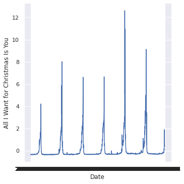
The “All I Want for Christmas is You” data looks how it should.
Eventually I want to start to use the pageview data from the in-linking pages to make a better forecast for this. There are 633 of these pages but I will also need to look at whether a page is a leading indicator by 30 days, 50 days etc. This quickly multiplies out to be a lot of potential regressor columns; I am nervous about chucking this amount of data at a regression algorithm and hoping it can figure out what is and isn’t important.
There are certainly situations where this would be a good approach but for this specific problem I don’t like it. There might be 2323 rows of data but there are only six Christmas peaks - and if I reserve one of them for testing then that only leaves five for training. This means there is a big risk of overfitting and the more regression variables I throw into the mix, the bigger this risk.
My plan here is to follow a two step process:
- Filter out a lot of the regression variables based on correlation value
- Setup the forecasting model so that it will only use a small number of them
There are a few different ways of doing step 2. Tensorflow supports “Structural Time Series” (more on this shortly) with a Sparse Linear Regression component.
SparseLinearRegression uses a parameterization of a Horseshoe prior to encode the assumption that many of the weights are zero, i.e., many of the covariate time series are irrelevant
Which sounds pretty close to what I want so let’s go with that for now.
Rather than diving straight into the deep end let’s start by making a simpler model so we can verify it works
import tensorflow_probability as tfp
import tensorflow.compat.v2 as tf

## Forgetting this line is my number one cause of mystery tf errors that I can't figure out
tf.enable_v2_behavior()
The “structure” in a structural timeseries describes how the timeseries evolves given certain parameters. For example, we might model the value at day t+1 as the value at day t plus a small amount of random noise. This is a “random walk” model and it can actually work pretty well for predicting things only 1 day ahead.
The parameters are estimated from historical data; in the above example the parameter to estimate is the variance of the random noise.
The first model I want to try is a bit more complicated than that. It is similar to how Forecast Forge works behind the scenes. There are three components:
- Two seasonalities; weekly and annual
- A trend component
The trend component looks a bit similar to the first random walk example:
level[t] = level[t-1] + slope[t-1] + Normal(0., level_scale)
slope[t] = slope[t-1] + Normal(0., slope_scale)
The main difference is that there is both a level and a slope both random walking around. This means that the model is slower to “change direction” than a random walk; if the slope is large and positive then it will take a few days for it to become negative and start trending the other way.
The weekly seasonality component will estimate an effect for each day. This is the same approach to seasonality that Tom Capper uses in his Google Sheets template on Moz.
The annual seasonality component is designed to be smoother than that. This is actually a weakness when forecasting “All I Want for Christmas is You” pageviews because the data is so “spikey” but I have picked this for three reasons:
- I don’t want to estimate 12 different monthly effects because the peak in pageviews is concentrated at one part of December. Adding an average effect for the whole month to whatever weekly seasonality there is won’t capture the 7 days before Christmas very well
- Estimating an effect for each of 365 days slows down the model fit quite a lot and eats RAM like it is going out of fashion. This way of modelling things also ignores any smoothness there might be in the data (e.g. the value for November 23rd is likely to be close to the values for November 22nd and 24th)
- This is most similar to what the Forecast Forge algorithm does which makes the forecasts more comparable
def build_model(observed_time_series):
  trend = tfp.sts.LocalLinearTrend(observed_time_series=observed_time_series)
  weekly = tfp.sts.Seasonal(
      num_seasons=7, observed_time_series=observed_time_series, name="week")
  annual = tfp.sts.SmoothSeasonal(
      period=365, frequency_multipliers=[1, 2, 3, 4, 5, 6])
  # The actual prediction is the sum of the above three components
  model = tfp.sts.Sum([trend, weekly, annual], observed_time_series=observed_time_series)
  return model
Let’s forecast for Christmas 2020 and see what it looks like against the actuals.
observed = normalised[normalised.index<"2020-11-09"]["All I Want for Christmas Is You"]
observed = list(observed)

model = build_model(observed)

# The below is mostly tensorflow voodoo
# The output will be a loss curve plot; we want to see that this converges before proceeding
variational_posteriors = tfp.sts.build_factored_surrogate_posterior(
    model=model)

num_variational_steps = 200

# Build and optimize the variational loss function.
elbo_loss_curve = tfp.vi.fit_surrogate_posterior(
    target_log_prob_fn=model.joint_log_prob(
        observed_time_series=observed),
    surrogate_posterior=variational_posteriors,
    optimizer=tf.optimizers.Adam(learning_rate=0.1),
    num_steps=num_variational_steps,
    jit_compile=True)

plt.plot(elbo_loss_curve)
plt.show()

# Draw samples from the variational posterior.
q_samples = variational_posteriors.sample(100)
WARNING:tensorflow:From /opt/conda/lib/python3.8/site-packages/tensorflow/python/ops/linalg/linear_operator_composition.py:182: LinearOperator.graph_parents (from tensorflow.python.ops.linalg.linear_operator) is deprecated and will be removed in a future version.
Instructions for updating:
Do not call `graph_parents`.
WARNING:tensorflow:From /opt/conda/lib/python3.8/site-packages/tensorflow_probability/python/distributions/distribution.py:342: MultivariateNormalFullCovariance.__init__ (from tensorflow_probability.python.distributions.mvn_full_covariance) is deprecated and will be removed after 2019-12-01.
Instructions for updating:
`MultivariateNormalFullCovariance` is deprecated, use `MultivariateNormalTriL(loc=loc, scale_tril=tf.linalg.cholesky(covariance_matrix))` instead.
WARNING:tensorflow:From <ipython-input-10-608bf49b6c8f>:15: StructuralTimeSeries.joint_log_prob (from tensorflow_probability.python.sts.structural_time_series) is deprecated and will be removed after 2022-03-01.
Instructions for updating:
Please use `StructuralTimeSeries.joint_distribution(observed_time_series).log_prob`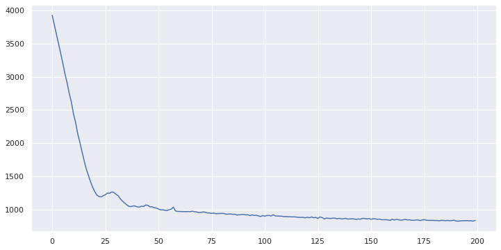
The model converges (yay!) so we can use the parameter samples from the posterior to get the forecast values
forecast_dist = tfp.sts.forecast(
    model,
    observed_time_series=observed,
    parameter_samples=q_samples,
    num_steps_forecast=53)

forecast_mean, forecast_scale = (
    forecast_dist.mean().numpy()[..., 0],
    forecast_dist.stddev().numpy()[..., 0])
Quick inspection of the forecast_mean data. We want to see values somewhere between 4 and 8 later in the series
forecast_meanarray([0.35945305, 0.48060617, 0.50919384, 0.5111362 , 0.6007148 ,
0.688883 , 0.7947957 , 0.9094128 , 1.0705427 , 1.1377562 ,
1.1766099 , 1.301028 , 1.4216119 , 1.5571762 , 1.698354 ,
1.8826438 , 1.9693264 , 2.023694 , 2.1594274 , 2.2869177 ,
2.424798 , 2.5635533 , 2.740567 , 2.8150437 , 2.8522348 ,
2.96582 , 3.0662289 , 3.1721685 , 3.2742407 , 3.4099848 ,
3.4387949 , 3.4261525 , 3.486002 , 3.5290675 , 3.5743883 ,
3.612922 , 3.6825888 , 3.6431928 , 3.5606399 , 3.5493193 ,
3.5204093 , 3.4934168 , 3.4597697 , 3.4578633 , 3.3479712 ,
3.1964653 , 3.1181912 , 3.02477 , 2.9361305 , 2.8441105 ,
2.787481 , 2.626873 , 2.428981 ], dtype=float32)Hmmm, possible a little low.
Pad these forecasted values out so we can compare them with the actuals in a plot
padded_forecast = np.pad(forecast_mean,(len(observed),0),constant_values=(np.NaN,))

forecast_df = pd.DataFrame({"forecast":padded_forecast
                           })
forecast_df["actuals"] = list(normalised["All I Want for Christmas Is You"] [:forecast_df.shape[0]])
forecast_df.index = normalised.index[:forecast_df.shape[0]]
forecast_df.index.name = "Day"
forecast_df = forecast_df[["actuals", "forecast"]]

sns.lineplot(data=forecast_df)
<AxesSubplot:xlabel='Day'>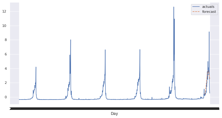
Not bad! It misses the big peaks but that is ok for now because the model doesn’t have anything in it to account for them.
Now back to doing some data-munging in preparation for the lagged regression.
First extend the index on the dataframe into the future - this is so there is “space” for the lagged regressors to go into. There is probably a better way of doing this, LMK if you know what it is.
from datetime import date
old_ix = pd.date_range(start=date(2015, 7, 1), end=date(2021, 11, 8), freq='D')
extended_ix = pd.date_range(start=date(2015, 7, 1), end=date(2021, 12, 31), freq='D')
normalised.index = old_ix
normalised = normalised.reindex(extended_ix)
The absolute minimum amount of lag we can consider is 53 days; this means the value on November 8th will tell us a bit about what happens on New Year’s Eve. I’ve decided the maximum to look at is 83 days; looking back earlier than October probably won’t give that much extra information.
So now make a dataframe with every page lagged between 53 and 83 days:
shifted = None
for i in range(53,83):
    x = normalised.drop(columns="All I Want for Christmas Is You").shift(periods=i).add_suffix("_"+str(i))
    if shifted is None:
        shifted = x
    else:
        shifted = pd.concat([shifted,x], axis=1)

shifted.columns
Index(['Justin Bieber_53', 'Millie Bobby Brown_53', 'Mariah Carey_53',
'Fifth Harmony_53', 'Jenna Dewan_53', 'Love Actually_53',
'Michael Bublé_53', 'Despacito_53', 'Tori Kelly_53',
'Hallelujah (Leonard Cohen song)_53',
...
'Colleen Madden_82',
'List of Tawag ng Tanghalan finalists (season 3)_82',
'List of top 10 singles for 2018 in Australia_82',
'The Masked Singer (Bulgarian season 1)_82',
'List of Billboard Global 200 number ones of 2021_82',
'Ngayong Pasko_82', 'Česko Slovenská SuperStar (season 4)_82',
'Mr. Vocalist X'Mas_82', '24 Hours (Agnes song)_82',
'We Were Born for This_82'],
dtype='object', length=18990)18990 is a lot of columns. Let’s reduce that number down by seeing which have a statistically significant correlation with “All I Want for Christmas is You”
from scipy.stats import pearsonr

sig_cols = []
for i in shifted.columns:
    nas = np.logical_or(np.isnan(normalised["All I Want for Christmas Is You"].values),
                        np.isnan(shifted[i].values.astype("float")))

    corr, pval = pearsonr(normalised["All I Want for Christmas Is You"].values[~nas],
                          shifted[i].values[~nas]
                         )
    if(pval < 0.05):
      sig_cols.append({"col":i, "corr":corr, "p":pval})

# View the top ten
sig_cols.sort(key=lambda x: -abs(x['corr']))
sig_cols[:10]
[{'col': 'Tawag ng Tanghalan (season 3, quarter I)_80',
'corr': 0.42718188064663565,
'p': 3.524046455470085e-100},
{'col': 'Tawag ng Tanghalan (season 3)_80',
'corr': 0.41963677515784387,
'p': 2.2040219582815046e-96},
{'col': 'Tawag ng Tanghalan (season 3)_81',
'corr': 0.4151538500141587,
'p': 3.9297134847417186e-94},
{'col': 'Tawag ng Tanghalan (season 3)_82',
'corr': 0.41496413323530373,
'p': 5.348570466557383e-94},
{'col': 'Tawag ng Tanghalan (season 3, quarter I)_81',
'corr': 0.38587368756325663,
'p': 1.6532525769584053e-80},
{'col': 'Tawag ng Tanghalan (season 3, quarter I)_79',
'corr': 0.37752700745584056,
'p': 6.1489592197905055e-77},
{'col': 'Tawag ng Tanghalan (season 3, quarter I)_82',
'corr': 0.36852002750662144,
'p': 4.9533722974120236e-73},
{'col': 'The X Factor: Celebrity_59',
'corr': 0.34727695650499074,
'p': 3.603730969714107e-65},
{'col': 'Tawag ng Tanghalan (season 3)_79',
'corr': 0.344126527727554,
'p': 2.114127129858737e-63},
{'col': 'The X Factor: Celebrity_58',
'corr': 0.31705212117051595,
'p': 4.591941729922087e-54}]“Tawag ng Tanghalan” is a Philippine singing competition which I’m guessing is similar to the X Factor (also listed in the top 10). It seems like these competitions start their TV runs in late Autumn and interest builds through until the final before Christmas - maybe so the winner can have a shot at a Christmas number one.
This means that interest and pageviews to their wikipedia pages start increasing through November so the lagged correlation with “All I Want for Christmas is You” appears strong. I’m guessing that “All I Want for Christmas is You” is also sung in the later stages of these competitions which is why the wikipedia pages are linked.
Worryingly, none of this is saying anything about what Mariah Carey is doing in November and wikipedia pages for new seasons of Tawag ng Tanghalan won’t be included in our data set but let’s plow on regardless.
def build_regressor_model(observed_time_series, regressors):
  trend = tfp.sts.LocalLinearTrend(observed_time_series=observed_time_series)
  weekly = tfp.sts.Seasonal(
      num_seasons=7, observed_time_series=observed_time_series, name="week")
  annual = tfp.sts.SmoothSeasonal(
      period=365, frequency_multipliers=[1, 2, 3, 4, 5, 6])
  regressors = tfp.sts.SparseLinearRegression(
       design_matrix=regressors, weights_prior_scale=0.01
  )
  model = tfp.sts.Sum([trend, weekly, annual, regressors], observed_time_series=observed_time_series)
  return model
training_regressors = shifted[[x['col'] for x in sig_cols]].to_numpy(na_value=0).astype("float32")
regressor_model = build_regressor_model(observed, training_regressors)
variational_posteriors = tfp.sts.build_factored_surrogate_posterior(
model=regressor_model)
# Build and optimize the variational loss function.
elbo_loss_curve = tfp.vi.fit_surrogate_posterior(
target_log_prob_fn=regressor_model.joint_log_prob(
observed_time_series=observed),
surrogate_posterior=variational_posteriors,
optimizer=tf.optimizers.Adam(learning_rate=0.1),
num_steps=num_variational_steps,
jit_compile=True)
plt.plot(elbo_loss_curve)
plt.show()
# Draw samples from the variational posterior.
q_samples = variational_posteriors.sample(100)WARNING:tensorflow:@custom_gradient grad_fn has 'variables' in signature, but no ResourceVariables were used on the forward pass.
WARNING:tensorflow:@custom_gradient grad_fn has 'variables' in signature, but no ResourceVariables were used on the forward pass.
WARNING:tensorflow:@custom_gradient grad_fn has 'variables' in signature, but no ResourceVariables were used on the forward pass.
WARNING:tensorflow:@custom_gradient grad_fn has 'variables' in signature, but no ResourceVariables were used on the forward pass.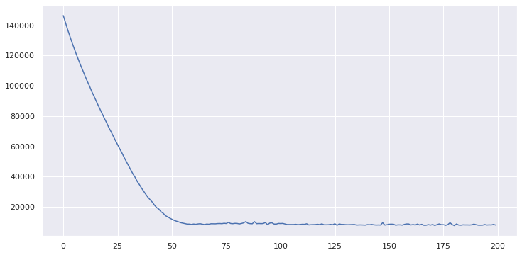
Now make the forecast
forecast_dist = tfp.sts.forecast(
    regressor_model,
    observed_time_series=observed,
    parameter_samples=q_samples,
    num_steps_forecast=53)
forecast_mean, forecast_scale = (
forecast_dist.mean().numpy()[..., 0],
forecast_dist.stddev().numpy()[..., 0])forecast_meanarray([0.4021134 , 0.26802546, 0.29915774, 0.35381198, 0.39239565,
0.4913519 , 0.62269664, 0.62460697, 0.6748683 , 0.8460419 ,
0.8314816 , 0.89810306, 0.9707965 , 1.1343668 , 1.271471 ,
1.3178807 , 1.3192046 , 1.4591802 , 1.5402098 , 1.6311107 ,
1.7568297 , 1.9190131 , 1.8498538 , 1.8599926 , 2.0212965 ,
2.163909 , 2.2679136 , 2.2723856 , 2.2320397 , 2.3305006 ,
2.2959707 , 2.3503718 , 2.5391078 , 2.5836945 , 2.656044 ,
2.612377 , 2.48579 , 2.6914563 , 2.6265645 , 2.6099665 ,
2.5055795 , 2.498663 , 2.4052846 , 2.3451033 , 2.2123523 ,
2.3186212 , 2.1818147 , 2.0509038 , 1.9053872 , 1.7598625 ,
1.5765525 , 1.5135591 , 1.4336597 ], dtype=float32)This seems way worse; peak value for the first forecast was 3.68 compared with 2.69 here
padded_forecast = np.pad(forecast_mean,(len(observed),0),constant_values=(np.NaN,))
forecast_df['Lagged regressors'] = padded_forecast
ax = sns.lineplot(data=forecast_df.tail(730), dashes=False, palette=["blue","green","red"], sizes=[1,10,10])
import matplotlib.dates as mdates
ax.xaxis.set_major_locator(mdates.MonthLocator(interval=3))
plt.show()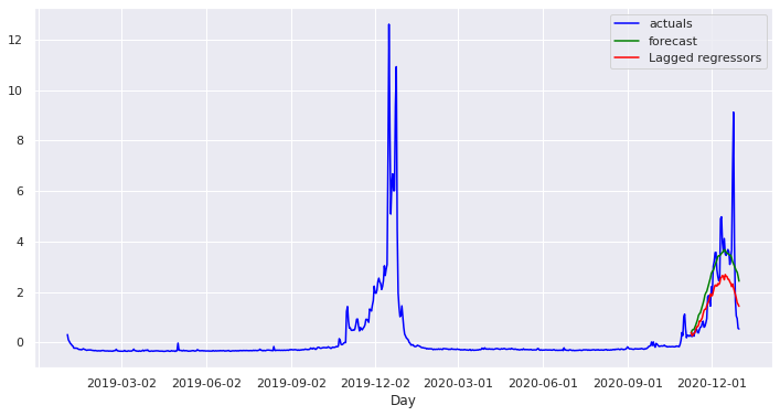
This is textbook overfitting :-(
Regressors that were predictive in December 2019 do not work so well in 2020 and the model has learned to rely more on the regressors than the seasonal components.
Let’s analyse this in a little more detail by looking at the regression coefficients
regs = q_samples['SparseLinearRegression/_weights_noncentered'].numpy().mean(axis=0)
from scipy import stats
stats.describe(regs)DescribeResult(nobs=9766, minmax=(-3.7824707, 5.50638), mean=0.0054672873, variance=0.11094342, skewness=2.445416212081909, kurtosis=42.830982132014604)sns.displot(regs)<seaborn.axisgrid.FacetGrid at 0x7fd35520a340>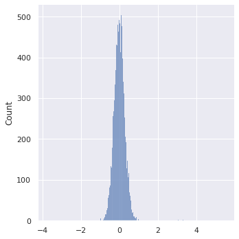
These are not what I expected! It is true that the regression coefficiants are tightly distributed around zero, but I was expecting it to be more obvious which of them were relevant and which weren’t. I think the SparseLinearRegression hasn’t worked the way that I wanted it to.
So to sum up there are two main problems here, they are kind of linked but each could happen alone too:
- I chucked a load of data at an algorithm expecting it to be able to figure out what was and wasn’t important
- The result was overfitted on the training set
Can I do better by manually choosing regressors?
Let’s look at only various lags for the Mariah Carey page.
cols = [col for col in shifted if col.startswith("Mariah Carey_")]
shifted_mariah = shifted[cols]
training_regressors = shifted_mariah.to_numpy(na_value=0).astype("float32")
regressor_model = build_regressor_model(observed, training_regressors)
variational_posteriors = tfp.sts.build_factored_surrogate_posterior(
model=regressor_model)
# Build and optimize the variational loss function.
elbo_loss_curve = tfp.vi.fit_surrogate_posterior(
target_log_prob_fn=regressor_model.joint_log_prob(
observed_time_series=observed),
surrogate_posterior=variational_posteriors,
optimizer=tf.optimizers.Adam(learning_rate=0.1),
num_steps=num_variational_steps,
jit_compile=True)
plt.plot(elbo_loss_curve)
plt.show()
# Draw samples from the variational posterior.
q_samples = variational_posteriors.sample(100)WARNING:tensorflow:@custom_gradient grad_fn has 'variables' in signature, but no ResourceVariables were used on the forward pass.
WARNING:tensorflow:@custom_gradient grad_fn has 'variables' in signature, but no ResourceVariables were used on the forward pass.
WARNING:tensorflow:@custom_gradient grad_fn has 'variables' in signature, but no ResourceVariables were used on the forward pass.
WARNING:tensorflow:@custom_gradient grad_fn has 'variables' in signature, but no ResourceVariables were used on the forward pass.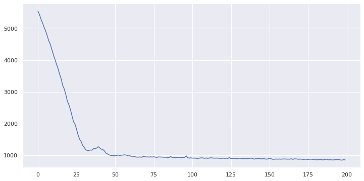
forecast_dist = tfp.sts.forecast(
regressor_model,
observed_time_series=observed,
parameter_samples=q_samples,
num_steps_forecast=53)
forecast_mean, forecast_scale = (
    forecast_dist.mean().numpy()[..., 0],
    forecast_dist.stddev().numpy()[..., 0])
padded_forecast = np.pad(forecast_mean,(len(observed),0),constant_values=(np.NaN,))
forecast_df['Mariah regressors'] = padded_forecast
ax = sns.lineplot(data=forecast_df.tail(730), dashes=False
, palette=["blue","green","red","purple"]
, sizes=[1,10,10])
import matplotlib.dates as mdates
ax.xaxis.set_major_locator(mdates.MonthLocator(interval=3))
plt.show()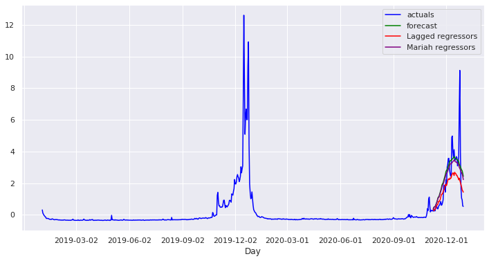
The result isn’t very different to the first attempt forecast; it looks like pageviews for “Mariah Carey” in November don’t tell you very much about what is going to happen in December.
I’m going to leave it here for the day, I hope this post has demonstrated two things:
- This stuff is hard. Being able to use fancy tensorflow models doesn’t necessarily make things any easier
- I don’t know enough about All I Want for Christmas is You to really drive this forward (or else it is just hard - see point 1)
If you've read this far and understood everything then you might not be in the target audience for the Forecast Forge Google Sheets Addon.
However, you probably have collegues who are! I would like to talk to them so please consider hooking me up with an introduction (fergie@forecastforge.com).
And feel free to email me with any other questions/comments you may have; I'd love to hear from you.