October 19, 2020

Extending Prophet for fun and profit - Part 1

Understanding the original implementation

Prophet is a general purpose forecast algorithm developed by Facebook. It is the main algorithm used behind the scenes for Forecast Forge (I’ll go into why I picked it some other time).

At the core of the Prophet code is a model written in a programming language called Stan. I am lucky enough to have some familiarity with Stan from other projects.

This model is where the interesting stuff happens; the rest of the Prophet code (R or python) is just around scaling and preparing data for input into this model and extracting the results at the end.

I’m going to assume for this that you are familiar with the process of using Prophet in R or Python. If you aren’t then read the getting started guide and fit a few forecasts. After that this all should all make a bit more sense.

We need to talk about Stan

Suppose you have some process that you are interested in and that this process is complicated enough that you want to model it as something random or stochastic. Calculating how long a car traveling at 70 miles per hour takes to go between two towns doesn’t fit into this category (it is too easy to model without) but something like whether or not a user converts on a website is; it is just too much to take into account all the variables like their mental state, what they had for lunch, whether their neighbor is slowing down your site by watching Netflix at the same time as they surf and all the rest.

Stan let’s you describe how this random process works (called a “generative model”) and then does some clever stuff in the background to figure out the parameters of the model. For example, a simple model for website conversion might be “the user converts at random with probability p and does not convert with probability 1-p”. Then Stan does Bayesian inference with this model and your data to tell you what the likely values of p are.

You might think this is a lot of work for something like estimating a conversion rate and you’d be right. Stan is more useful when the model gets more complicated and I will show you an example of this in this post.

The Prophet model

In this post I will go through the existing Prophet Stan model. Then, in future posts I will discuss how it can be changed and modified for different things.

You can view the current model on github.

Stan is kind of an old fashioned language in that variables need to be declared in advance and there is very little flexibility in the order of code. Rather than start at the top and work down we will start at the end - at the absolute key part - and then work out.

The model

The most important part of the model is on line 136:

y ~ normal(
  trend
  .* (1 + X * (beta .* s_m))
  + X * (beta .* s_a),
  sigma_obs
);

This describes how the y values (i.e. the thing we are trying to forecast) vary depending on the things they depend on.

If I rewrite it like this it should be easier to see what is going on:

y ~ normal(
  trend
  .* multiplicative_regressors
  + additive_regressors,
  sigma_obs
);

So the y values are normally distributed around a trend, multiplied by some multiplicative_regressors and added to some additive_regressors. The variance is sigma_obs; a small value of sigma_obs will mean the model fits the y values used in training very closely so the predictive interval for the forecasted values will be narrower. sigma_obs is estimated from the data during model fitting.

Let’s unpack the regressors a bit more. Both of them have the form X * (beta .* s_?) where s_? is either s_a or s_m.

The s_? variables are provided by the user when they specify for each regressor whether it is multiplicative or additive. Each s_? is a vector with the same length as the number of regressors. For regressor number i, s_a[i] is 1 if it is an additive regressor and s_m[i] is 1 if it is a multiplicative regressor.

The beta values are regression coefficients. In Stan .* means elementwise multiplication so element i in the vector beta .* s_a is beta[i] * s_a[i].

Because of how we defined s_a earlier this means it is zero unless it is an additive regressor. So X * (beta .* s_a) means only the additive regressors are included in the additive component. The same goes for the multiplicative regressors as s_m.

X is a matrix containing the values of the regressor variables; again, the user provides this before fitting starts.

If this looks very similar to the maximum likelihood method for doing a regression that is because it is! One of the things that amazes me about Prophet is that it can work so well across so many different things with such a simple model.

I guess “just use regression!” is a meme for a reason.

The trend part is perhaps the most interesting and the most complicated. The simplest version of the Prophet model (no saturation) has a piecewise linear trend; where the trend is linear between fixed changepoints provided by the user.

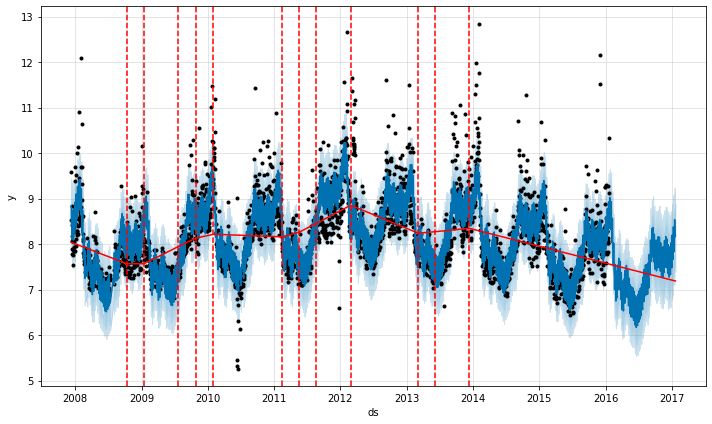
In the above image the vertical dotted lines are the changepoints and the straight red lines are the linear trend between them.

This is one of the limitations of Prophet - if you’re trend doesn’t look like this then the model won’t fit it very well. E.g. if you are undergoing true exponential growth. But, on the other hand, regression has a wide range of uses so I tend not to worry about this too much.

Parameters

Now we’ll skip back a few lines to the parameters block on line 108.

The parameters are the things we are hoping the model will learn when we fit it. For example in a two dimensional linear regression y = m*x +b the parameters are m and b.

In this model the parameters are:

parameters {
  real k;                   // Base trend growth rate
  real m;                   // Trend offset
  vector[S] delta;          // Trend rate adjustments
  real<lower=0> sigma_obs;  // Observation noise
  vector[K] beta;           // Regressor coefficients
}

k and m are parameters for the initial trend; they correspond to m and b in my example above. They state what the trend line does up until the first changepoint.

delta is a vector of values, each one of which is how much (and in what direction) the trend changes at each changepoint. For example, if k is 0.5 and delta[1] is -0.3 then after the first changepoint the slope of the trend is 0.5-0.3=0.2.

sigma_obs and beta we have already seen in the model section. beta is a vector of regression coefficients and sigma_obs describes how much randomness (or variation from the model) there is in the data.

Note the S and the K in the declaration of delta and beta; this says there are S changepoints and K regressors. i.e. the numbers here are flexible and can be changed by the user.

One thing you won’t be seeing here, that might seem like a strange omission is that there are no parameters around seasonality or holidays. These are both important features of the Prophet model so what gives?

In both cases these are added as regressor columns.

For holidays a regressor column is created with zeros in every row except for the date of the holiday. This is often not what you want - in this case you need to create a custom regressor column with an appropriate date range for your holiday. The effect of the holiday is then determined by the matching beta[i].

How can cyclical seasonal effects be fitted like this? Doesn’t linear regression only deal with straight lines?

The above gif shows what happens as you add together trigonometric functions called “fourier terms”. By picking the right coefficients you can approximate any continuous periodic function with enough fourier terms. By default Prophet adds 10 fourier terms for annual seasonality and 10 for weekly seasonality to the regression matrix. These are generated in R/python before the data is sent into Stan.

This limit to 10 terms limits the “spikiness” of the seasonality that Prophet can fit. This is one of the reasons why the fit in my Easter pageviews example isn’t so good.

The coefficient for each fourier terms is part of the beta parameter and it is fitted in the same way.

Priors

Now jump to line 128 which is where the model priors are defined.

You can think of priors as a way stating what we expect the values of the parameters to be before we have seen any data. Then Bayesian updates are performed as the model is fit using the data - the end result is that the output is some combination of what we knew beforehand and what the data says.

Knowing how best to pick priors to match what is already known about a problem is a whole big area of discussion that I can’t do justice to here. Instead I will talk through the priors that Prophet uses:

//priors
k ~ normal(0, 5);
m ~ normal(0, 5);
delta ~ double_exponential(0, tau);
sigma_obs ~ normal(0, 0.5);
beta ~ normal(0, sigmas);

normal(0,5) is a normal distribution centered on zero with variance five. The values in the data are scaled before they are sent to Stan so that everything is between 0 and 1. This means this prior is relatively “uninformative”; it covers a wide range of reasonable values and we aren’t constraining what the values might be very much. This is like saying “I don’t know what the value will be, but I’m pretty sure it won’t be really big or really small”.

k and m define the trend at the start of the training data; so we are saying we don’t really know what these will be but that they are probably not extreme.

The prior for delta is very different; the double_exponential distribution. This means we expect the values of delta to be zero (or very close to it). delta describes how much the trend changes at a changepoint; by using this prior we are saying that the trend probably won’t change; so the data must contain strong evidence for a trend change for there to be one in the end result.

The prior for beta is similar to that for k and m. sigma can be specified by the user (see the data block); the default is 10 so this is an even more vague/uninformative prior than on the trend.

This tells us a bit more about how Prophet might fit extreme data.

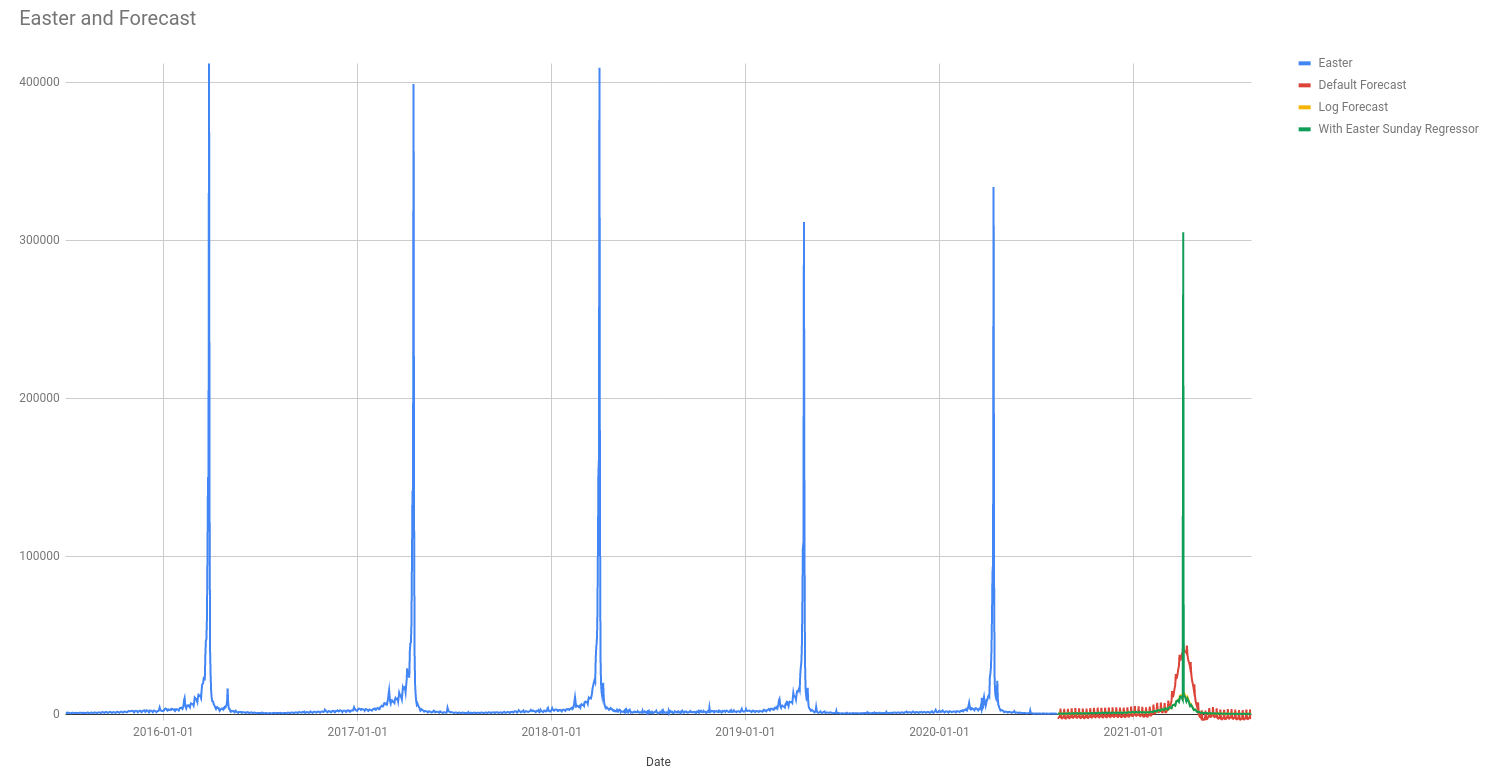
For example, the above image shows Prophet trying to fit the daily pageviews for the Wikipedia page about Easter. The green line is from a forecast where there is a regressor added for Easter Sunday (it is zero everywhere except Easter Sunday).

It seems weird to me that the predicted value for Easter Sunday is lower than the previous five years. This isn’t because Prophet is predicting a negative trend for Easter; we know that that isn’t part of the model. Instead it is because all regressor coefficients have the same prior normal(0,sigma). Specifying a different sigma just for this regression coefficient might give a better result. You can do this in Prophet but unfortunately not in Forecast Forge at the present time.

There is a lot more in the prophet.stan file but this covers the most important parts of what it does. The rest is more how it does it which is less important for understanding the strengths and weaknesses of the model.

---