Tips for reducing the width of the predictive interval
In my last post I talk about how you can use a forecast to measure the impact of a some kind of change (e.g. Google rewriting your title tags in the SERP). One of the main difficulties you might find with this is that the width of the predictive interval is too wide to conclude that a change has had a positive/negative effect with XX% probability.
What do you do if your best guess is that the test has a positive outcome but you aren’t 95% sure? Will Critchlow has written about this kind of issue which they sometimes see at Search Pilot. Will has a set of recommendations they use in this situation based around the mantra “we’re doing business, not science” which is an important rule to remember (unless you are a scientist!).
You can just follow this advice and not worry too much about whether your before/after comparison is inconclusive or not. But you might also be able to improve your forecast model to reduce the width of the predictive interval; this can give you more confidence in your decision (I’m talking about confidence as an emotion here, not as a probability of being right; although the two are linked!) and, as a bonus, you get a better forecast that you can use for other things too.
So here is my best advice for reducing the width of the predictive interval when making an SEO forecast.
1. Account for large spikes
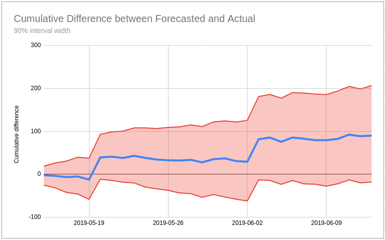
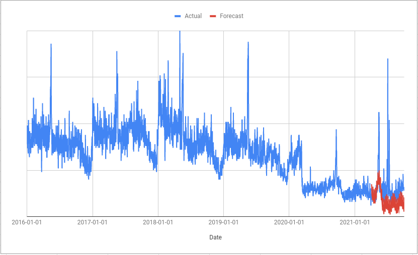
When you compare a forecast with what actually happened often you will see large spikes in your actual values that are not reflected in the forecast. These are the main thing that will cause the forecasting algorithm to give you a wide predictive interval.
Ask yourself what happened on those days and then, if you have an answer, see if you can turn it into a regressor column so that the forecasting algorithm can “know” what was going on for those days.
To anthropomorphise the algorithm a bit, without this regressor column all it can see is that on some days the actual values are way higher or way lower than it would otherwise expect. It assumes that this variation is random so it learns to expect a similar amount of random variation in the future. This is what gives you a much wider predictive interval.
2. Control for the things you aren’t interested in
The main problem with running a before/after test is that other things can change between the before period and the after period. For example, I have spoken to people who have been in the unfortunate postion of having had their search rankings change at the same time as covid lockdowns were introduced. In this situation, if you use the approach to forecasting the impact of lockdowns that I’ve recommended before then the forecasting algorithm cannot tell the difference between the changes because of lockdown and the changes because of the ranking change. In practice this means the algorithm assumes that when lockdowns end, your rankings will return to whatever they were before.
When specifically looking at the SERP title tag rewrite change the same situation is possible; you are interested in the impact of new title tags on click through rates but what if rankings change at the same time and that is what causes the click through rate to change?
You can control for this in a few ways:
- Add a regressor based on search console data that takes into account the number of impressions your site is getting and the expected click through rate (this sounds hard, but I think some SEO’s probably have a model for this already)
- Use something like the Sistrix visibility
index
which does a similar thing but with much less work for you!
[Thanks to Sam Underwood for this tip]
3. Watch out for step changes
When making a forecast, Forecast Forge is estimating three things:
- The underlying trend
- Seasonality
- The impact of any regressors you have added
These things are then added together to make the final prediction. The predictive interval width is determined by the uncertainty in the above estimates and the estimated random variation for your metric; we know that real life will never perfectly match up with our forecast so the algorithm also needs to estimate the size of these random differences.
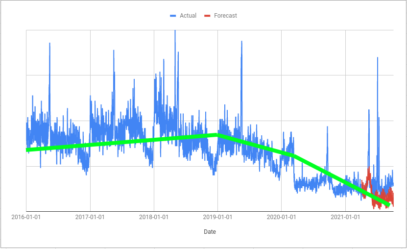
The trend compnent is what is known as “piecewise linear”. This means that it is made up of a series of straight lines joined togther.
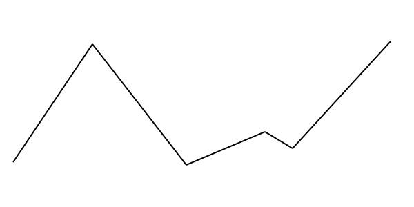
This kind of trend line is hard to fit around “step changes” in your data.
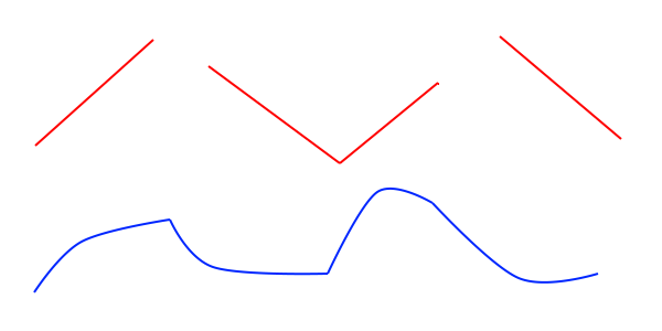
The algorithm can end up interpreting a step change as a change in trend:
The trend is then extraploated out into the future; you can see in the example above that the green trend line doesn’t take into account the step change and instead assumes it is the start of a decline. This is one reason why the forecast is lower than the actual values.
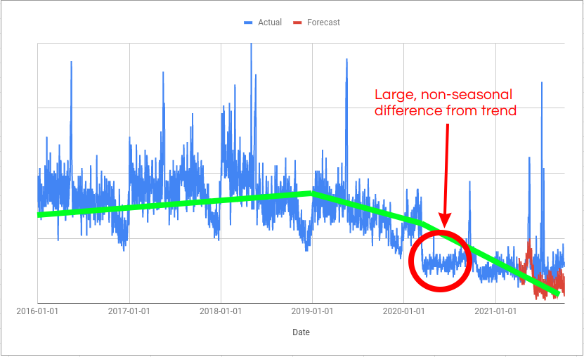
On the day of the step change (in this example, it is the start of Covid in the UK) there is a large gap between the trend and the actual values. And this gap persists until the trend “catches up” with the step change. The algorithm knows this variation isn’t seasonal because it hasn’t happened in previous years so it assumes it is random variation; this is what increases the width of the predictive interval.
The soloution to this is to add a regressor column with different values before and after the step change; 0 and 1 is simple and works well but any two values will work.
Of course, if the step change occurs at the same moment as the change you are trying to evaluate then don’t do this!
All of these tips are generally useful for making better forecasts but they are also useful for making more sensitive before/after tests.